Background
Motivations
One of the key insights in data analysis is that "data has shape". While this shape depends on how the data is embedded and represented, it is often the case that the shape of the data is a key feature of the data itself. For instance, when working with time series data, the data may have a periodic shape due to time's cyclical nature. To better exploit this feature of the data, topological data analysis (TDA) uses tools such as persistent homology to quantify these features in a mathematically rigorous way.
Persistent homology is a tool from algebraic topology that assigns combinatorial structures (simplicial complexes) at varying resolutions of the data, usually calculated through some filter function, much like a level function in Morse theory. The homology of these simplicial complexes are then computed, giving a measure of the \( k \)-dimensional "holes" present in the data, and the persistence of features in this homology is tracked as the resolution of the data changes. Intuitively, a hole which is present at all resolutions is likely a robust feature of the data, while a hole which appears and disappears quickly is likely noise. These features can then be used to cluster data, reduce dimensionality, or otherwise analyze the data.
Machinery
Suppose \( X \subset \mathbb{R}^d \) is the dataset, usually called a point cloud since \( \lvert X \rvert < \infty \). The first step in the usual TDA pipeline is to choose a filter function that assigns each interval \( [0,\varepsilon) \) a simplicial complex \( \Delta_\varepsilon \). In a lot of cases, the filter function is chosen to be the usual Euclidean distance as this distance is physically meaningful to the data itself. In this case, for each \( \varepsilon \geq 0 \), set \[ X_\varepsilon = \bigcup_{p \in X} B(p, \varepsilon), \] where \( B(p, \varepsilon) \) is the open ball of radius \( \varepsilon \) centered at \( p \), to get a filtration of the dataset \( X \). Then, assign a simplicial complex \( \Delta_\varepsilon \) to each \( X_\varepsilon \) by taking, for example, the Vietoris-Rips complex of \( X_\varepsilon \). We then get a series of inclusions as \( \varepsilon \) increases, i.e., \( X_{\varepsilon_1} \subseteq X_{\varepsilon_2} \) whenever \( \varepsilon_1 \leq \varepsilon_2 \). The key insight is to that these inclusions induce maps in homology, and the persistence of these maps is what is tracked.
In some sense, the homology of the simplicial complexes \( \Delta_\varepsilon \) is a measure of the "holes" present in the data at resolution \( \varepsilon \). The persistence of these holes can be summarized through a persistence diagram or equivalently through a barcode diagram.
- Definition. A feature (actually a homology class) which first appears in \( \Delta_b \) is said to be born at time \( b \). Similarly, a feature which first vanishes in \( \Delta_d \) is said to die at time \( d \).
-
Definition.
A persistence diagram is a multiset of points in the plane, where each point \( (b,d) \) represents a feature that is born at time \( b \) and dies at time \( d \).
This can be transformed into a lifetime diagram via the transformation \( (b,d) \mapsto (b, d-b) \).
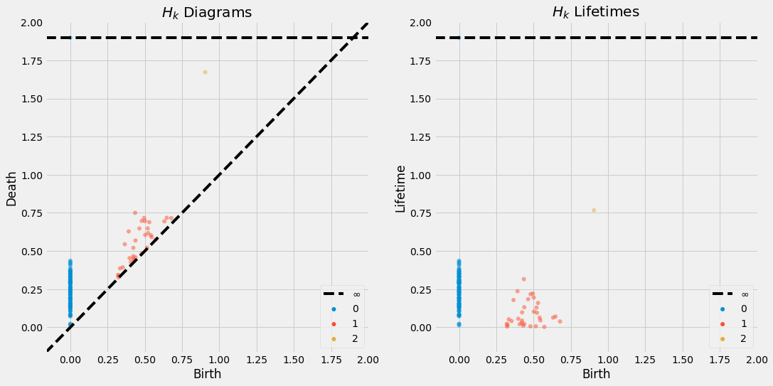
The persistence and lifetime diagrams of a point cloud sampled from a sphere. -
Definition.
A bardcode diagram is a multiset of intervals \( (b,d) \) where each interval represents a feature that is born at time \( b \) and dies at time \( d \).
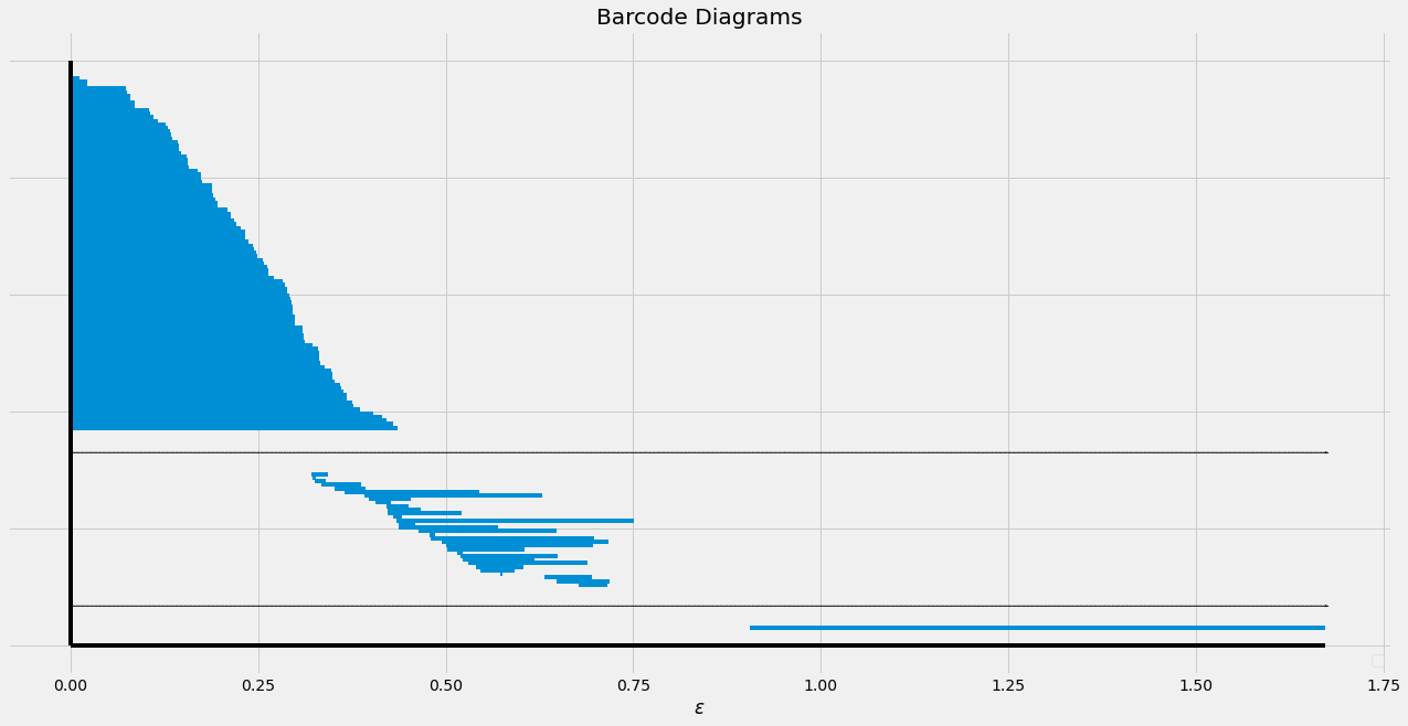
The barcode diagram of a point cloud sampled from a sphere.
Since a feature cannot die before it is born, the persistence diagram is always above the diagonal \( y = x \) and the bars in the barcode diagram always have positive length. Intuitively, points farther from the diagonal in the persistence diagram (or longer bars) should encode more persistent features in the data. The persistent diagram and barcode diagram thus summarize the persistent topological features which seem to be present in the data.
Results
Bootstrapping computations
Joint with Jordan Eckert.Computing persistent homology is a computationally intensive task which is intractable for relatively small datasets (e.g., \( \lvert X \rvert \approx 10^4 \)). To mitigate this, we can use bootstrapping techniques to estimate the persistent homology of the data from smaller samples of the data. More precisely, we can sample \( X \) multiple times to get a collection of smaller datasets \( \{ X_k' \}_{k=1}^N \) (abusing the notation from above), compute the persistent homology of \( X_k' \), and then aggregating these results to get an estimate of the persistent homology of \( X \). Since \( \lvert X_k' \rvert \ll \lvert X \rvert \), the persistent homology of \( X_k' \) is computationally feasible.
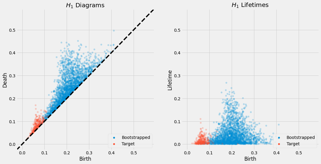
Experimentally, we have found that this technique seems to reasonably approximate the persistent homology of the full dataset, but with some scale factor on the persistence diagram and with some important features sometimes being missed. The scale factor is likely due to a uniform sampling of the dataset yielding points which are sparse across the dataset, so the "time" at which features appear is artificially inflated as there is a greater distance between points. The missing features are likely due to the fact that the bootstrapping technique is not guaranteed to sample the dataset uniformly, and so some features may be missed entirely, or the scale of the feature is misaligned with the scale of the sample.